Using Map data in R

Maps are useful things and R is a useful thing, so it would seem a natural useful thing to get them to work together.  However, maps are far more complex that we might think and dealing with them in R can be a bit interesting.

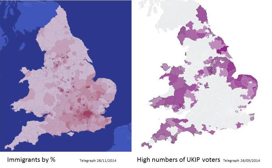
I started looking for map data to follow up a discussion on the correlation between votes for a far-right wing party (UKIP) and lack of exposure to immigrants. The recent UK elections have provided a wealth of data, and figures like these suggest that there may be a correlation.

Data for voting patterns in May 2013 can be obtained from the electoral commission at http://www.electoralcommission.org.uk/our-work/our-research/electoral-data
Data for the recent census can be retrieved from http://www.nomisweb.co.uk/census/2011/KS204EW which gives the country of birth at a local authority level.

The Electoral data is an Excel file that is nicely split and formatted in a way that makes it difficult to read directly into R. However, by spending a few minutes editing out the subheadings and copying the regional names to a new column, I have a tab-delimited file that gives me the electoral votes by local authority.

origins<-read.csv('bulk.csv',stringsAsFactors=F)
origins$geography <- toupper(origins$geography)
names(origins)[c(5:16)]<-c('All','UK','England','Northern.Ireland','Scotland','Wales','UK.Other','Ireland','EU','EU2001','EU.New','Other')

The Nomis data gives a good CSV file with appropriate headings, though these needed some rewriting to be more friendly in R. All the Local Authority names (origins$geography) have been capitalised to match the electoral data.

votes<-read.table('EPE-2014-Electoral-data.txt', header=T, sep='\t')
votes$Local.Authority<-toupper(votes$Local.Authority)
regions<-merge(votes,origins, by.x='Local.Authority', by.y='geography')

So this gives us the votes data and this can then be merged with the regional census data.
A plot is straightforward, as is a regression analysis.

UKIPvote<-100*regions$UKIP/regions[,4]
NonUK<-(regions$All.y-regions$UK)*100/regions$All.y
plot(UKIPvote~NonUK, xlim=c(0,60), ylim=c(0,60), xlab='% non-UK born',
       ylab='UKIP vote (%)', main='Anti-immigrant vote vs population composition')
abline(lm(UKIPvote~NonUK), col=2)

summary(lm(UKIPvote~NonUK))

Call:
lm(formula = UKIPvote ~ NonUK)

Residuals:
     Min       1Q   Median       3Q      Max 
-12.0187  -3.6868  -0.1728   3.3297  14.5318 

Coefficients:
            Estimate Std. Error t value Pr(>|t|)    
(Intercept) 34.17057    0.67626   50.53   <2e-16 ***
NonUK       -0.49421    0.03117  -15.86   <2e-16 ***
---
Signif. codes:  0 ‘***’ 0.001 ‘**’ 0.01 ‘*’ 0.05 ‘.’ 0.1 ‘ ’ 1

Residual standard error: 4.956 on 116 degrees of freedom
Multiple R-squared:  0.6843, Adjusted R-squared:  0.6816 
F-statistic: 251.4 on 1 and 116 DF,  p-value: < 0.00000000000000022

Looks good to me - fear of strangers leads to reactionary politics.
Now to recreate the maps. This is where it starts to get interesting.

Map data for the UK at local authority boundary level is not readily available. Datasets are at ward level or higher level regions. So I will need to read in the ward data and merge the local authorities so I can plot the electoral data. The frame of reference is latitude and longitude for the polygon coordinates.

ONS census ward (merged wards) data is available from http://www.ons.gov.uk/ons/guide-method/geography/products/census/spatial/2011/index.html. This downloads as a zip archive that unpacks into a folder containing multiple files with the same root filename. These are ARCGIS SHAPEfile format. Get the full resolution file as the generalised one fails to merge wards properly.

The R package maptools is used to read them. Whilst you are at it also install the libraries rgeos, rgdal and gpclib to process the data. Set your session to the directory containing the data files and read them in.

library(maptools)
library(rgeos)
library(rgdal)
library(gpclib)

GPClib is proprietary and licensed for non-commercial use. To enable it type

gpclibPermit()

wards <-readShapePoly("CMWD_2011_EW_BGC")

This gives the ward boundaries and these can be plotted readily using the shapefile objects plot command.

plot(wards) #this could take a while so try plotting a selection
plot(wards[1:20])

This datafile contains the local authority name. However, we need to merge the datafiles to local authority. That can be done by unifying individual polygons (dissolving in shapespeak) to anew boundary list where the id is the local authority name.

lamap <-unionShapePoly(wards, wards$LAD11NM)

But this gives an error.
So I process the data local authority by local authority until I find the error
for(x in levels(wards$LAD11NM)){
  try( {
    cat(x);
    lamap<-unionSpatialPolygons(wards[wards$LAD11NM==x,],    
        wards$LAD11NM[wards$LAD11NM==x]);
  })
}

This lists all the LA names as we go and the errors so it is clear to see which ones are providing problems. It does take a long time to process Wales - the coastline is quite challenging.

In total there were 5 local authorities who showed errors. I now have two options:

1. Fix the errors
2. Work round them by plotting everything except the problem ones and plotting them as wards.

I give up with 1.
With 2 I can use the R subset command to select the good wards and merge those. That leaves the bad wards to plot on top of them afterwards.

goodwards<-subset(wards, !(wards$LAD11NM== 'Bridgend'| wards$LAD11NM=='Gwynedd'| wards$LAD11NM=='Isle of Anglesey'| wards$LAD11NM=='Newcastle-under-Lyme'| wards$LAD11NM=='Oxford'))
badwards<-subset(wards, wards$LAD11NM== 'Bridgend'| wards$LAD11NM=='Gwynedd'| wards$LAD11NM=='Isle of Anglesey'| wards$LAD11NM=='Newcastle-under-Lyme'| wards$LAD11NM=='Oxford')

Now I can merge the good ones.

lamap<-unionSpatialPolygons(goodwards, goodwards$LAD11NM)

And plot

plot(lamap)
plot(badwards, add=T)

Now we'll work on colouring them by the data.

And I should update this for the EU referendum..